Normal Distribution
Suppose we have a dataset representing the heights of adult males in a population. The heights of 1000 individuals are measured, and the data follows a normal distribution with a mean of 175 centimeters and a standard deviation of 6 centimeters.
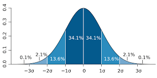
The normal distribution can be represented graphically as a bell-shaped curve. The mean of 175 centimeters will be the center of the curve, and the standard deviation of 6 centimeters will determine the spread of the data.
Using the properties of the normal distribution, we can make several observations:
Symmetry: The normal distribution is symmetric, so the curve will be centered at the mean of 175 centimeters.
Bell-shaped curve: The probability density function of the normal distribution will produce a bell-shaped curve when graphed. The curve will be highest at the mean and gradually decrease towards the tails.
Empirical Rule: According to the empirical rule, approximately 68% of the data falls within one standard deviation of the mean, 95% falls within two standard deviations, and 99.7% falls within three standard deviations.
For this example, we can use the mean and standard deviation to make probabilistic statements about the dataset: Approximately 68% of the individuals have heights between 169 centimeters (175 - 6) and 181 centimeters (175 + 6).
Approximately 95% of the individuals have heights between 163 centimeters (175 - 2 * 6) and 187 centimeters (175 + 2 * 6).
Approximately 99.7% of the individuals have heights between 157 centimeters (175 - 3 * 6) and 193 centimeters (175 + 3 * 6).
These statements provide a range within which the heights of the majority of individuals in the population are expected to fall, based on the characteristics of the normal distribution.
Understanding the normal distribution allows us to make probabilistic inferences, calculate probabilities, and analyze data by standardizing values using z-scores.
The normal distribution is widely applicable in statistical analysis and serves as an important tool in various fields, such as quality control, hypothesis testing, and population modeling.

Enroll Now
- Python Programming
- Machine Learning